There are a lot of value distributions functions. However in real world we have three most useful: even, normal and linear. Let's review these three models and build test data arrays for.
All test data generation software products by DTM soft has built-in engine that provides $RFloat function. This function produces floating point numbers in user defined range and with defined precision i.e. digits after decimal point. The function has optional parameter for generated value distribution.
In the article we'll deal with DTM Data Generator for Excel due to visualization of results reason. However, there are no differences in the random number generation function calls with another software titles of the mentioned product line.
For our experiments we'll generate 1000 values per set between 0.0 and 1.0 with 3 digits precision. There is base function call for this purpose: $RFloat(0,1,3,%.3f). "%.3f" is a format string means number with 3 digits after dot only.
Next, we'll split our 0 to 1 range to 10 subsets and calculate how many values in each of them has been generated: 0 to 0.1, 0.2 to 0.2, ... 0.9 to 1.0. The built-in function FREQUENCY of the Microsoft Excel is must suitable to calculate these values.
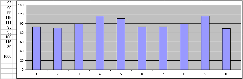
Even Distribution
By default this function produces random set of numbers with even distributions. In other words we expect same number of values in each of interval. Actually it is not exact equal for small so arrays due to random nature of values. At the column we can see number of values generated by the software in each interval and 1000 is total number of the items in the complete set.
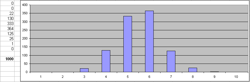
Normal Distribution
The second probability distribution is normal or Gaussian. In this case we expect, that middle of our interval 0 to 1 i.e. 0.5 is most probably generated value and 0 and 1 are least probable. To setup this model we have to pass "Normal" parameter to $RFloat function as described in the manual. Also, we'll pass "dispersion" value 0.25 to make our set more visual: $RFloat(0,1,3,%.3f,Normal,0.25)
As you can see intervals 0 to 0.2 and 0.8 to 1 have probability about 0. Most of data are located near mean value 0.5:
Under the Hood
To create sequence of random values with normal distribution the test data generation engine uses BoxľMuller transformation. This algorithm converts even distribution of the random values to Gaussian one. There is sample C++ code without details:
	V1 = 1.0-double(rand())/16380.0;	/* 2 random values between -1 and 1 */
	V2 = 1.0-double(rand())/16380.0;

	s = V1*V1+V2*V2;
	return V1*sqrt(-2*log(s)/s);		/* value to be generated without shift to mean */
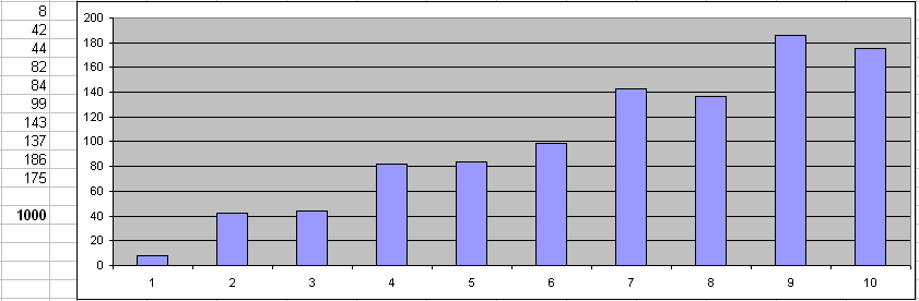
Linear Distribution
The last distribution today is linear. In this case we expect that probability grows from left side of the interval (0.0) to the right side (1.0). As you can see the first subset has 8 values only when the last one contains 175 values.
How to change linear distribution's properties? The simplest way is to use $RFloat call as a part of some expression that changes slope of the graph to required value.
Well, but hot to generate integer values with required probability? The function can create integer values as well if you produce 0 as precision and provide another interval instead of [0;1]. For example: $RFloat(0,200,0,%3.0f,Normal,3) will provide integers around 100.
How to generate a sequence of test data values with custom distribution? Please contact our support team to discuss your case. If it is not possible with built-in engine we'll glad it to engine for you.